Low Resolution Sea Ice Drift product (OSI-405)
In the context of the first Continuous Development and Operation Phase (CDOP-1), a sea ice drift product was introduced in the Ocean and Sea Ice SAF product's portofolio. It is based on low resolution (10-15 km) Passive and Active Microwave instruments (PMW and AMW) such as SSMIS, AMSR-E, ASCAT, etc...
The spatial resolution is 62.5 km on a Polar Stereographic Grid similar to the one used for the other OSISAF sea ice products. It is a 2 days (48 hours) ice drift dataset processed on a daily basis, which means that a product file measuring sea ice motion between 16th and 18th of February is available already on 19th of February. The 48 hours duration is possible thanks to the CMCC (Continuous MCC) method that was developped and implemented at the OSI SAF High Latitude centre. Single-sensor products as well as a multi-sensor dataset are made available.
1. Introduction and FAQ
How should I cite this dataset?
This dataset shall be referred to as the low resolution sea ice drift product of the EUMETSAT Ocean and Sea Ice Satellite Application Facility (OSI SAF, https://osi-saf.eumetsat.int).
The motion tracking methodology (CMCC) is published and shall be cited as Lavergne, et al. (2010):
Which satellite sensors are processed?
The sensors and channels used are SSMIS (91 GHz H&V pol.) on board DMSP platform F17, ASCAT (C-band backscatter) on board EUMETSAT platform Metop-A, and AMSR-2 on board JAXA platform GCOM-W.
What is the spatial resolution of this product?
The low resolution sea ice drift product is a gridded dataset. The grid has 62.5 km spacing on a Polar Stereographic projection mapping. Definitions for the projection parameters can be found in the NetCDF files as well as in the Product User's Manual.
What is the time-span of this product?
Two days (48 hours). This is the time delay between the start and the stop time of the motion described by one vector. For comparison, the merged products from IFREMER/CERSAT is a 3 days lag dataset while the AMSR-E product by the same data centre is 2 days (using 89 GHz channels).
Several datasets are distributed every day, which one should I use?
The OSI SAF low resolution sea ice drift product is indeed composed of several single-sensor products and one multi-sensor analysis, every day. They are all at the same spatial resolution , on the same grid and with a 48 hours time-span.
The multi-sensor (aka merged, multi-oi) is intended for users requiring a spatial covering dataset. In this product, missing vectors are indeed interpolated from the neighbours and each vector is computed from the individual single-sensor products. In this merging process, however, some level of aliasing and averaging is to be expected that slightly degrade the quality of the dataset.
For this reason, single-sensor products are also distributed. They can be more accurate than the merged product, especially concerning the start and stop time of the motion vectors. However, it is not unlikely that some vectors will be missing or, in case of interrupted data flux, that all data will be missing. Those products are thus intended for more advanced users or assimilation techniques that can cope with missing data. The optimal assimilation setup would be to use all the single-sensor products in building the model analysis.
A product file is empty, what happened?
Two possible answers:
- Missing input data: In case of interrupted data link with the satellite operating centres, or failure of the satellite sensor, no input swath data are available for processing of sea ice drift data, resulting in an empty grid.
- Summer period: Since May 2017, the OSI SAF sea-ice drift product provides motion vectors during the summer season (1st May to 1st October in the NH grid, 1st November to 1st April for SH grid) based on the 18.7 GHz imagery of the GCOM-W1 AMSR2 sensor. Before that date, and in case of temporary or definitive failure of the AMSR2 instrument, the product grid is empty during the summer period.
In both cases, the status_flag dataset in the product file indicates the reasons for missing data.
What is the legend used for the quicklooks?
Quicklooks for the product can be viewed from this page: https://osisaf-hl.met.no/quicklooks-1prod
Scaling of vectors
For easier visualization, the magnitude of the vectors was scaled by 3. Since the spacing between the base point of two arrows is 62.5 km, vectors that are drawn with a length of 62.5 km are really corresponding to a drift of 20.8 km (distance between the start point and stop point after 48 hours).
Dates associated to the displacements
Quicklooks are indexed on the stop date of the displacement. A quicklook displayed for date January, 10th 2010 is really corresponding to the displacement from the 8th to the 10th of January.
Colour codes for the vectors
| Colour | Vectors | |
|---|---|---|
| Nominal quality. | Corresponds to flag 30 | |
| The vector was computed as spatial interpolation of the neighbours. | Merged product only, corresponds to flag 22 | |
| The vector was retrieved by using its neighbouring vectors as spatial constraint. | Single-sensor products only, corresponds to flag 21 | |
| The vector was computed using a smaller image block. | Single-sensor products only, corresponds to flag 20 | |
| Colour | Background | |
| land | Operational Sea Ice Edge product | |
| open water | " | |
| open ice | " | |
| closed ice | " | |
| unclassified (coastal areas) | " | |
Do you have a similar ice motion product for Antarctic regions?
Yes! Since April 2013, we are distributing a Southern Hemisphere (SH) product, that can be accessed from the same FTP locations. It is only available during SH winter, that is from April 1st to October 31st.
I do not fancy NetCDF, do you have other formats?
The processing chain is currently only producing NetCDF files. Please let us know (contact) if you need another format.
2. Algorithms
2.1 Daily maps
Daily maps of satellite signal are aggregated from swath data at the High Latitude processing centre. The average sensing time is also computed in order to access an estimate of the start and stop time of each drift vector. A Laplacian filter is applied on those daily images for enhancing and stabilizing the features to be tracked (similar to the strategy developed at IFREMER/CERSAT).
|
(a) |
(b) |
(c) |
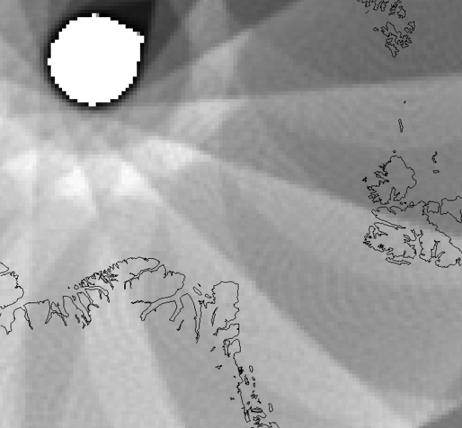
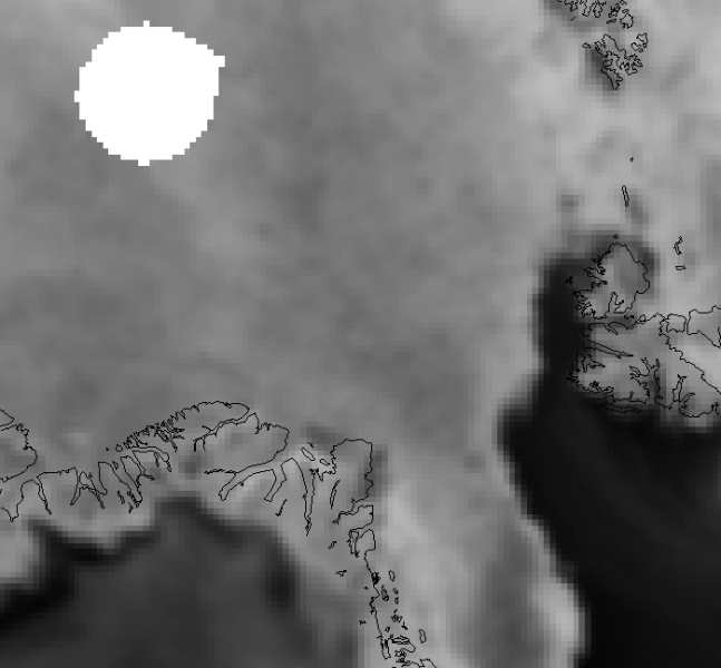
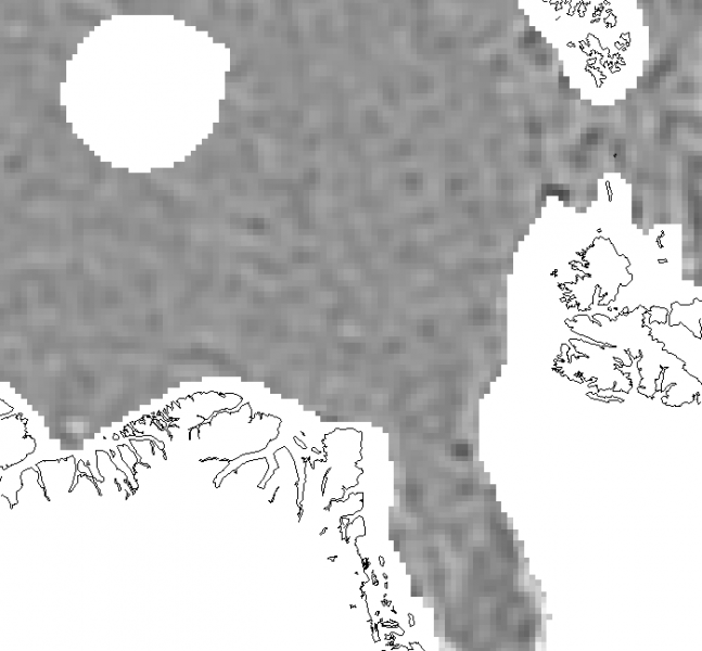
The ice mask used is the OSI-402 ice edge product. Two Laplacian filtered images, with central time two days apart from each others are the input data for the ice motion tracking algorithm (next section).
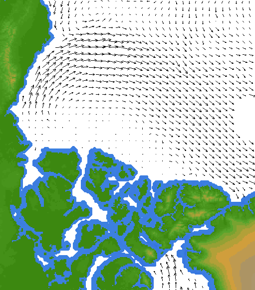
2.2 Motion tracking algorithm
Based on the well known Maximum Cross Correlation (MCC) method, the Continuous MCC (CMCC) relies on a continuous step for optimizing the components of the motion vector, located at the maximum of the cross-correlation function between a reference and a candidate blocks. In practice, virtual image pixels are interpolated from neighbouring pixels in each candidate block. The maximum point is search for in the 2D plane of valid (dx,dy) components by a "simplex" Nelder-Mead algorithm.
The main effect of using the CMCC is the removal of the quantization noise (aka tracking noise), which has hindered the retrieval of ice motion over short time spans from the same sensors. Quantization noise is responsible for MCC vector fields to look quantized, with a poor angular homogeneity and large areas with exactly the same vector. It is an artifact of the MCC algorithm.
|
(CMCC) |
(MCC) |

Strategies for optimally merging the information content of two polarization channels into a unique motion vector, as well as for filtering and correcting the few erroneous vectors that arise after the motion tracking steps have also been implemented. The main filtering is based on spatial consistency constraints and is built so that to allow for correcting drift vectors and thus avoiding to empty the product grid.
2.3 Multi-sensor merging strategy
The multi-sensor product aims at:
- Gaining confidence on the ice motion by a synergetic use of several instruments
- Avoid missing data
To meet those objectives, the merging methodology is based on two steps, applied one after the other. First, all grid locations where at least one single-sensor product has a valid motion vector are assigned a merged motion vector, as a weighted average of the available estimates. Weights are related to the standard deviations of single-sensor datasets, as documented below in the validation section. For the time being, there is no auto-correlation between the grid cells.
The first merging step does not allow for filling in the cell positions where no vectors were processed by any of the single-sensor products. Such areas are present in every product files, for example in the Polar observation hole. The second merging step thus consists in a spatial interpolation of the remaining missing vectors from the motion vectors in the closest vicinity. Interpolated vectors are explicitely marked in the status_flag dataset, should a specific user want to discard them.
Although this strategy fulfills the goals introduced above, a certain level of dynamic is bound to be lost and aliased during the merging process. As a consequence, rapidly changing drift patterns, such as when a low pressure system travels over sea ice, might be better described by single-sensor datasets than in the multi-sensor product.
3. Validation
Validation of OSISAF low resolution sea ice drift dataset was conducted in the Arctic against in situ drifters. Trajectories were usually made available as hourly (and sub-hourly) GPS records for an optimum temporal collocation. The validation exercise extended over 3 Arctic winters: 1st October to 30th April 2006-2007, 2007-2008 and 2008-2009. Statistical results and graphs document an excellent agreement between the various OSISAF low resolution sea ice drift datasets and the reference data.
Trajectories from the Ice Tethered Profilers (ITP), the Tara schooner and the Russian manned stations NP-35 and NP-36 (AARI) were processed during this validation exercise.
Matchup statistics are summarized in the following table and graph:
| Dataset | avg_Ex [km] | avg_Ey [km] | sdev_Ex [km] | sdev_Ey [km] | corr_ExEy | N |
|---|---|---|---|---|---|---|
| AMSR-E (Aqua) | -0.10 | -0.10 | 2.70 | 2.77 | -0.03 | 3977 |
| SSM/I (F15) | -0.07 | -0.02 | 4.10 | 4.01 | 0.02 | 4218 |
| ASCAT (Metop-A) | -0.17 | -0.24 | 4.71 | 4.47 | +0.01 | 3668 |
| Merged | -0.12 | -0.27 | 3.65 | 4.05 | +0.04 | 4707 |
|
|
|
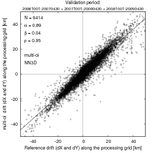
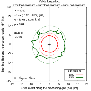
Out of those validation studies, the dataset derived from AMSR-E only compares best to ground truth. The Merged dataset has somewhat degraded quality but also much fewer data gaps. More details on the validation methodology can be found in the Validation Report.
Monthly validation statistics are regularly updated on the Validation and Monitoring page.
4. Documentation and links
The following documentation is available, further describing the OSI-405 ice drift product.
5. References
5.1 Peer-reviewed articles
| [1] | Lavergne, T., Eastwood, S., Teffah, Z., Schyberg, H. and L.-A. Breivik (2010), Sea ice motion from low resolution satellite sensors: an alternative method and its validation in the Arctic. J. Geophys. Res., 115, C10032, doi:10.1029/2009JC005958. at AGU site |
5.2 Reports, proceedings, etc...
| [1] | Lavergne, T., Low resolution sea ice drift Product User's Manual - v1.8. Technical Report SAF/OSI/CDOP/met.no/TEC/MA/128, EUMETSAT OSI SAF - Ocean and Sea Ice Satellite Application Facility, July 2016. |
| [2] | Lavergne T., Validation and monitoring of the OSI SAF low resolution sea ice drift product - v5. Technical Report SAF/OSI/CDOP/met.no/T&V/RP/131, EUMETSAT OSI SAF - Ocean and Sea Ice Satellite Application Facility, July 2016. |
| [3] | Lavergne, T., Eastwood, S., Schyberg, H., and L.-A. Breivik. Ice drift monitoring from low resolving sensors: an alternative method and its validation against in-situ data. Report MERSEA_WP02_METNO_STR_005_1A, MERSEA - Marine EnviRonment and Security for the European Area, October 2008. |
| [4] | Lavergne, T., Algorithm Theoretical Basis Document for the OSI SAF low resolution sea ice drift product - v1.3. Technical Report SAF/OSI/CDOP/met.no/SCI/MA/130, EUMETSAT OSI SAF - Ocean and Sea Ice Sattelite Application Facility, May 2016. |
| [5] | Lavergne, T., Eastwood, S., Röhrs, J., Schyberg, H., and L.-A. Breivik. Sea ice motion from space: an alternative method and its validation in the Arctic. proceedings to the ESA Living Planet Symposium, Bergen (Norway), 28 June - 2 July 2010. PDF, poster |